for controlling and monitoring Dual-space Iterative Processes
combining direct-method phasing of
OASIS with other protein crystallographic programs
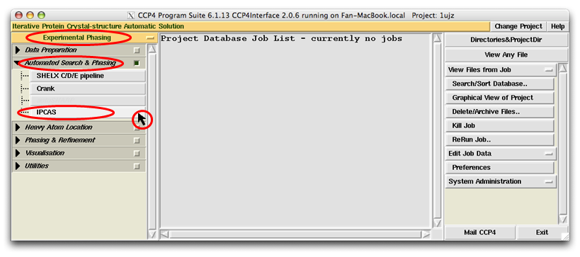
IPCAS GUI consists of two parts, the control panel and the monitoring board.
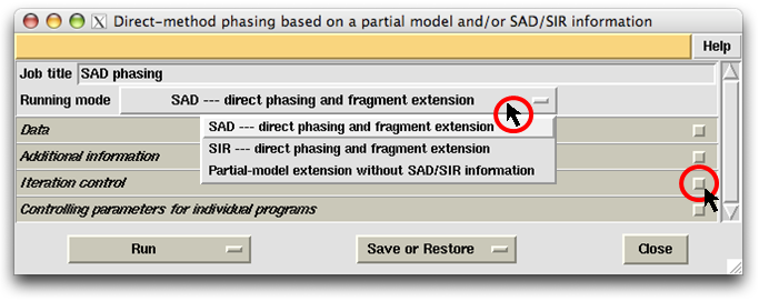
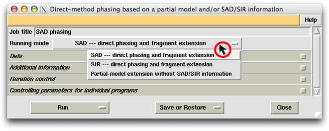
The control panel begins with a job title and the running-mode selector (see the figure above).
Below the running-mode selector there are four subframes entitled respectively "Data",
"Additional information", "Iteration control" and "Controlling parameters for
individual programs". Each subframe can be opened or closed by clicking the subframe-title bar
or the widget on the right of it.
By default the first two subframe are opened while the other two are closed (see the figure below).
The user should fill up slots in the first two subframes to provide IPCAS necessary information for
running a job. Some default controlling parameters are listed in the last two subframes. If the user wish
to change any default controlling parameters, just open the subframe and make corresponding changes.

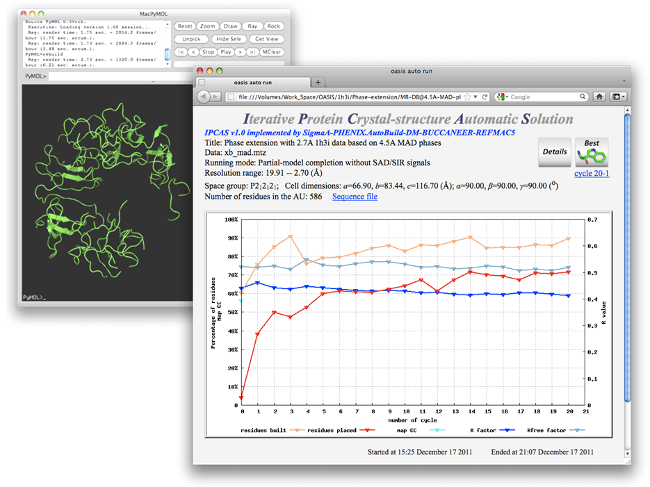
The monitoring board (see the following figure) is a graphical monitor of a single IPCAS job and will be brought up automatically once the job starts. If for some reasons the board does not appear, or when the job has completed and the board is closed, it can be called back at:
(Work directory) /auto_oasis_data/0_html/monitor.html
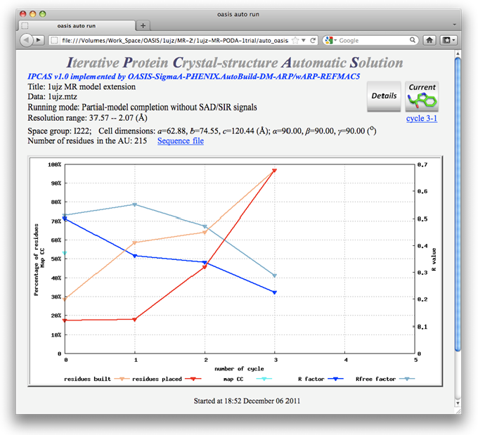
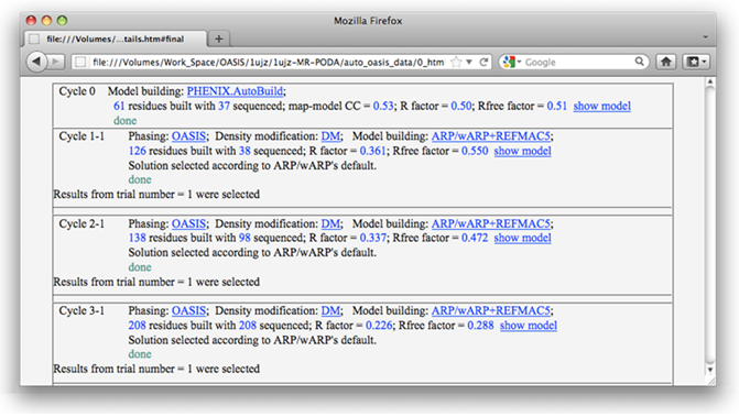
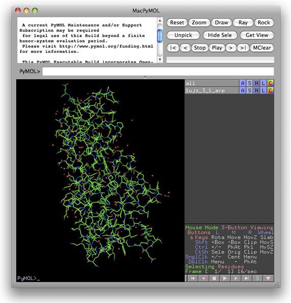
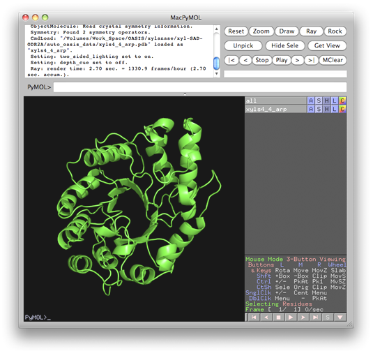
On the monitoring board, there is a Gnuplot graph displaying the progress of the iteration process. Besides, the user can click on the button "Details" near the top right to get a detailed list for all finished cycles (see the figure below) or click on "Sequence file" above the Gnuplot graph to check the sequence. By clicking the button next to "Details", the current model (stored in a PDB file) will be opened and can be manipulated by PyMOL [DeLano, W.L. (2002). The PyMOL Molecular Graphics System (San Carlos, CA: DeLano Scientific)] (see the figure after the next one).
Back to TOP
Back to OASIS.html
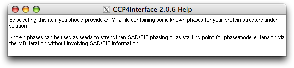
The first thing to do on the control panel is to select the "Running mode". As is seen in the following figure, there are three choices available. The first two are dedicated to SAD/SIR phasing and partial-structure model extension making use of SAD/SIR information. The third choice covers a number of different jobs. First, it can perform a molecular replacement by searching an MR model using the programs Chainsaw and Phaser, then followed by the MR iteration involving direct-method phasing, density modification and model building/refinement. Secondly, given a partial model (even fragments) from whatever sources, it can perform a model completion by the MR iteration leading to nearly the complete structure in favourable cases. Finally, given a set of known phases at low resolution (below 4Å), it can perform a dual-space phase extension leading to nearly the complete structure in favourable cases.
Suppose the running mode SAD is selected, then the default Job title will be "SAD phasing". The user can replace this title with other character strings.
There are two major processes running under IPCAS. The first named SAD/SIR iteration, which is for SAD/SIR phasing and fragment extension; The second named MR iteration, which was originally designed for MR-model completion. But actually it is used for a wide variety of fragment extension in the absence of SAD/SIR information. The flowchat of these two processes are shown below.

Back to TOP
Back to OASIS.html
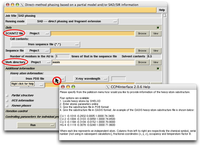
After choosing the "Running mode", the user should specify the location of diffraction data file (in sca or mtz format) in the slot next to the label "SCA/MTZ file". The user should also specify a "Work directory", which by default will be a subdirectory named "oasis" under the CCP4 directory "Project" (see the following figure). The "Work directory" will keep all intermediate files for the whole iterative process.
Hovering the mouse on some buttons, slots or widgets, a small yellow message board saying "Right click for help" may appear (see the button "from PDB file" in the following figure). Right clicking on that item, you can get an online help in the pop-up window. Pop-up-window messages form an important part of the OASIS tutorials. Be sure to close the existent message window before you are trying to get another one. More details of the control panel will be given together with examples in the next section. New users of OASIS and/or IPCAS are recommended to read "Examples" one by one carefully.
Back to TOP
Back to OASIS.html
| Sample | Xylanase S-SAD data |
Tom70p Se-SAD data |
Rpe Hg-SIR (PCMS) with 8Å MIR phases |
E7_C-Im7_C complex native data |
Set 7/9 Fobs (remote) with 4.5Å MAD phases |
| Space group | P21 | P21 | H3 | I222 | P212121 |
| Unit-cell | a=41.19, b=67.18, c=50.88Å; β=113.47o |
a=44.89, b=168.77, c=83.41Å; β=102.74o |
a=189.80, c=60.10Å; γ=120o | a=62.88, b=74.55, c=120.44Å |
a=66.90, b=83.44, c=116.70Å |
| Resolution limit (Å) | 1.8 | 3.3 | 2.8 | 2.1 | 2.7 |
| X-rays | 1.49Å synchrotron | 0.9789Å synchrotron | 1.5418Å (CuKα) | Synchrotron | Synchrotron |
| Number of residues in the AU |
303 | 1086 | 668 | 215 | 586 |
| Heavy atoms in the AU | 5 S + 1 Cl (?) | 24 Se | 7 Hg | ||
| Bijvoet ratio (<|ΔF>|/< F >) (%) |
0.56 | 4.3 | |||
| Solvent content (%) | 37 | 47 | 58 | 57 | 48 |
| Data multiplicity | 15.9 | 3.3 | |||
| Reference | Acta Cryst. D59, 1020 (2003). By courtesy of Dr. Z. Dauter |
PDB code: 2GW1. By courtesy of Prof. B.D. Sha |
JMB 262, 721 (1996). PDB code: 1LIA. By courtesy of Prof. D.C. Liang |
PDB code: 1UJZ. | PDB code: 1H3I. By courtesy of Dr S.J. Gamblin & Dr. B. Xiao |
All the following examples were calculated under Mac OS X version 10.5.8 with
CCP4 version 6.1.13
ARP/wARP version 7.0.1
BUCCANEER version 1.4.0
IPCAS version 1.0
OASIS version 4.2
PHENIX version 1.7.2-869 and
REFMAC version 5.5.0109
All calculations for the following examples were performed automatically from the start to the end
without manual intervention.
All necessary data files for rerunning the following examples are stored in the directory
~/ipcas1.0/examples/.
Rerunning the following examples under different computing enviroment may lead to similar but not exactly
the same results.
This example represents one of the most difficult cases in SAD phasing owing to the low Bijvoet ratio (0.56%) and low solvent content (0.37). However the sample protein can be solved by a default run of SAD iteration starting from the sca file and ending at a nearly complete structure model. Necessary input items in the control panel are shown in the following figure.
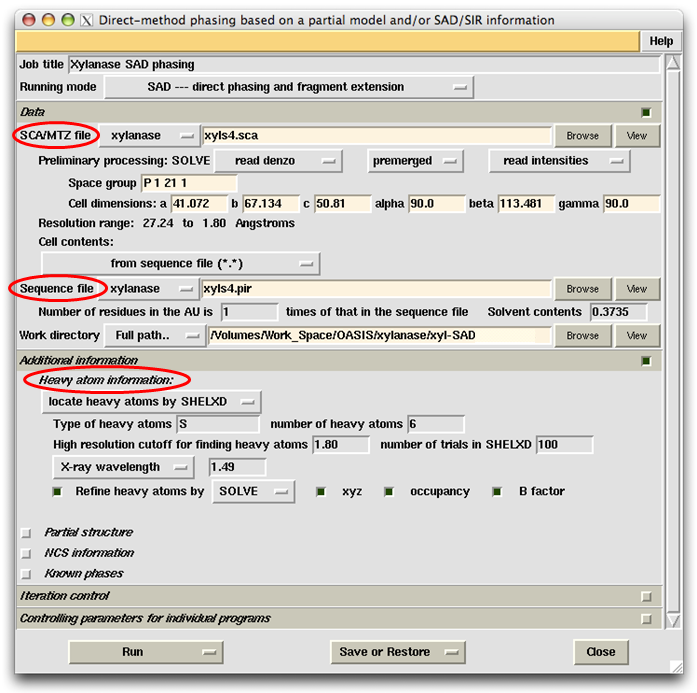
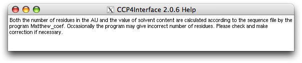
First, in the slot next to the label "SCA/MTZ file", the user should specify the location of input data (reflections) file. Here it is the file xyls4.sca which is in the project directory "xylanase". The space group symbol, unit cell parameters and resolution range will be automatically extracted and displayed on the control panel. Then the user should specify the sequence file. Here the file is xyls4.pir. Once the sequence file was input, a message window will appear as is shown in the following figure. Be sure to check and make necessary correction accordingly. Finally the user should provide the heavy atom (anomalous scatterer) information as shown on the control panel.
The last two subframes on the above control panel are closed. This means that parameters in the two subframes are already set according to the IPCAS's default. If you open the closed subframes, you can check and change any of the parameters if necessary (see the following figure).

Should you have a question on a particular parameter, please try hovering the mouse on it and, if the "Right click for help" message appears, then by right clicking the item you can get an explaination from the popup-window message. Some examples are shown below. On the subframe "Iteration control", right click the button next to the label "Model building by", you will get the following message:
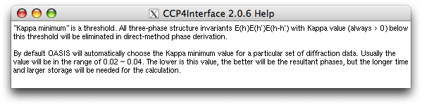
On the subframe "Controlling parameters for individual programs" and within the "OASIS parameters", right click the item "auto" in the slot next to the label "Kappa minimum", you will get the following message:
Right clicking on the item "Not forcing cos(deltaPhi)'s ..." you will get:
.png)
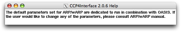
For "ARP/wARP parameters", right clicking the widget on the left of it you will get the message:
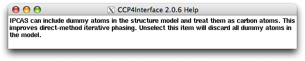
Right clicking on the item "Include dummy atoms ..." you will get:
To start running the job, on the control panel click the button "Run" and select "Run Now". This will also bring up the monitor. The graph in which records the progress of iteration. The yellow and red curves denote respectively percentages of the number of built and the number of sequenced residues against the number of residues in the structure. Values are shown on the left ordinate. The green and blue curves denote respectively the variation of Rfree and R, values of which are shown on the right ordinate.

Detailed results for each cycle can be listed by clicking the button "Details" near the top right of the monitor.
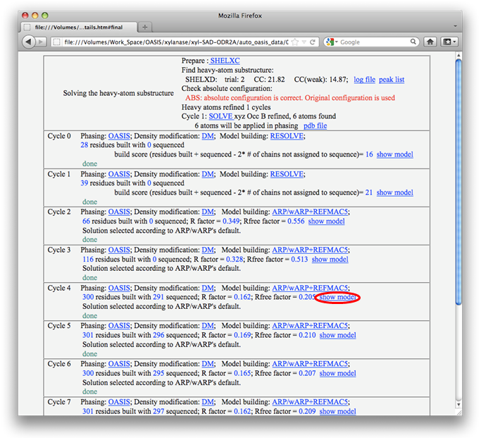
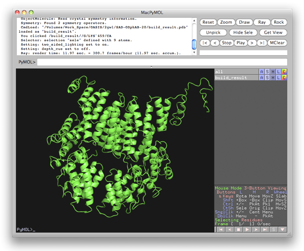
From results shown in the above two figures, it is seen that nearly complete structure models have been built from cycle 4 onward. Models can be displayed and manipulated online with the program PyMOL by clicking the links "show model". The resultant model of cycle 4 is shown below.
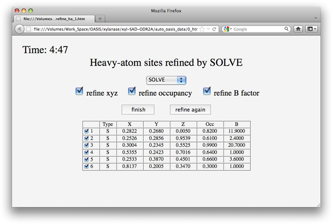
In this example, according to settings on the control panel, heavy atoms should be first located by SHELXD and then refined by SOLVE. Upon finished running of SHELXD, a message board will appear as is shown below telling you what IPCAS will do next, i.e.
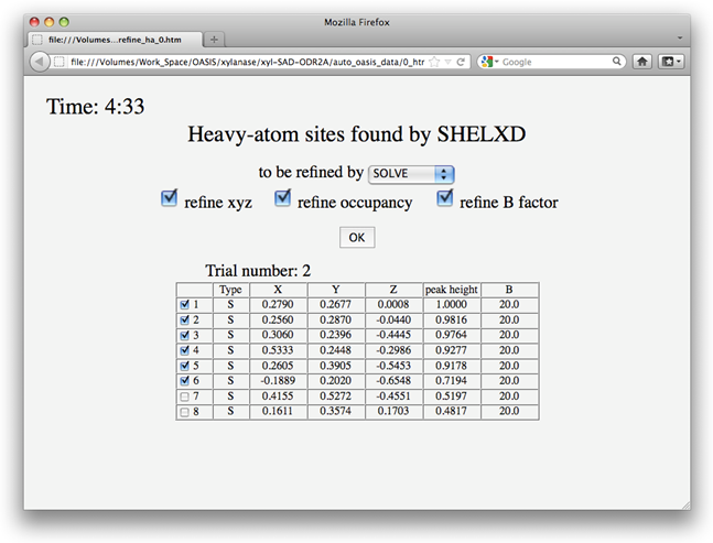
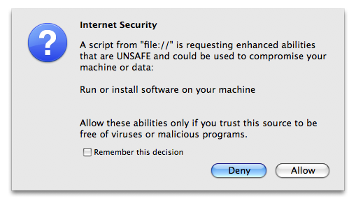
You have 5 minutes to change the selections (including the program for refinement) on the board. After that, IPCAS will automatically continue to run with selections on the board that appeared at the last moment. You can force IPCAS to continue immediately by clicking on the OK button and on the following message board selecting "Allow".
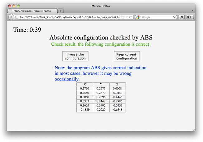
Before starting the refinement, IPCAS will check the absolute configuration of the heavy-atom substructure using the program ABS. Unlike that running two parallel jobs in SAD phasing by using both enantiomorphic heavy-atom substructures, IPCAS runs a single job based on the choice of the program ABS. In most cases ABS makes the right decision. However, if the user find that the job is getting into trouble, be sure to try the other enantiomorph. The user can make his/her own choice on the message board (see the following figure), which will appear upon finished running the program ABS.
After one cycle of refinement, a message board will appear as the following. The user can decide either to finish the refinement and go on to the next step, or to do one more cycle of refinement. In case of no response in 5 minutes, IPCAS will assume the "finish" and go on to the next step automatically.
Back to TOP
Back to OASIS.html
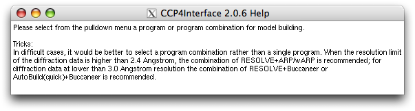
This example represents one of the most difficult cases in SAD phasing owing to the low resolution (3.3Å) and low redundancy (3.3). For model building at low resolution (~3Å), both PHENIX.AutoBuild and Buccaneer show very good performance. In our experience, the combination of the two is particularly suitable of building models from electron density maps below 3Å resolution. The controlling parameters are set accordingly as shown in the following.
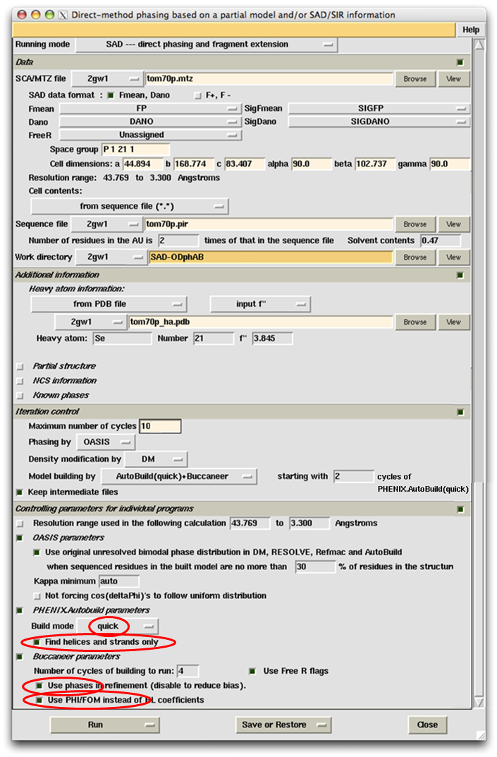
Online helps are also provided for parameters of PHENIX.Autobuild and Buccaneer. Right click an item marked with a red oval on the above panel will bring up the corresponding explaination as shown below.
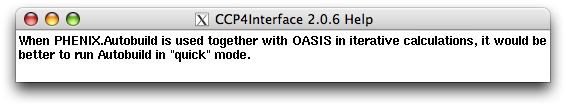
Right click "quick":
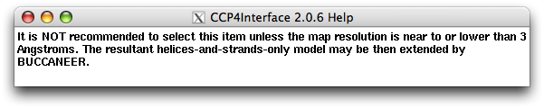
Right click "Find helices and strands only":
Right click "Use phases ...":
Right click "Use PHI/FOM instead of ...":
Results:
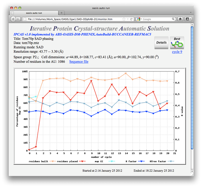
20 cycles of SAD iteration were recorded in the above monitoring board. The best structure model (shown below) came from cycle 9. While it is not brilliant, but still acceptable. On the other hand, a nearly complete structure model can be obtained by the combination of SAD iteration and MR iteration, see the 5th example.
Back to TOP
Back to OASIS.html
Phased SIR (or SAD) iteration is one of the new features of OASIS4.2. The SAD/SIR iteration has beeen extended to enable the use of a set of known phases. The effect of this extension can be seen in the present example.
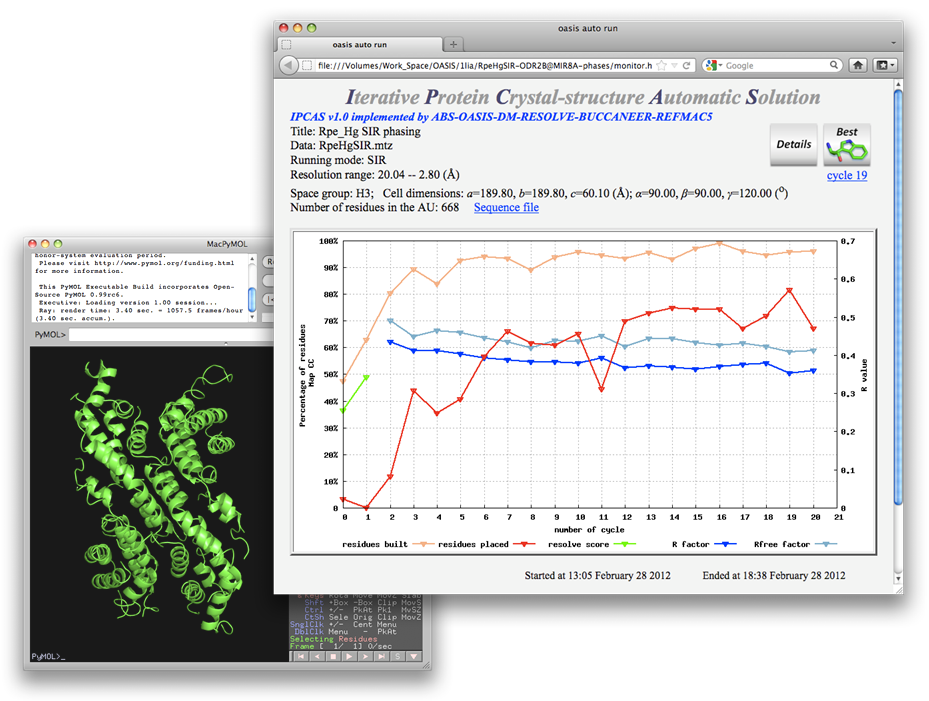
The protein Rpe was originally solved by the MIR method with four heavy-atom derivatives. The mercury (PCMS) derivative has been taken for the present test. Conventional SIR iteration with data of the PCMS derivative and the native protein was simply unsuccessful as is seen from the monitoring board (upper right) and the "best model" (lower left) in the following figure.

Adding known-phase information into the above calculation while keeping other controlling parameters unchanged, a reasonable result can be obtained as will be seen in the following. The known-phase information is a set of 8Å MIR phases. Data and parameters used in the calculation are shown on the control panel below.

Online helps are provided for the use of "Known phases", see those items marked with red ovals.
Right click the widget on the left of "Known phases":
Right click the button under "Known phases" or the slot next to the button:
Right click the short slot below the label "PHIB" and on the left of "% of known phases ...":

The resultant structure model can be further improved to nearly the complete structure by the combination of SIR iteration and MR iteration, see the 6th example
Back to TOP
Back to OASIS.html
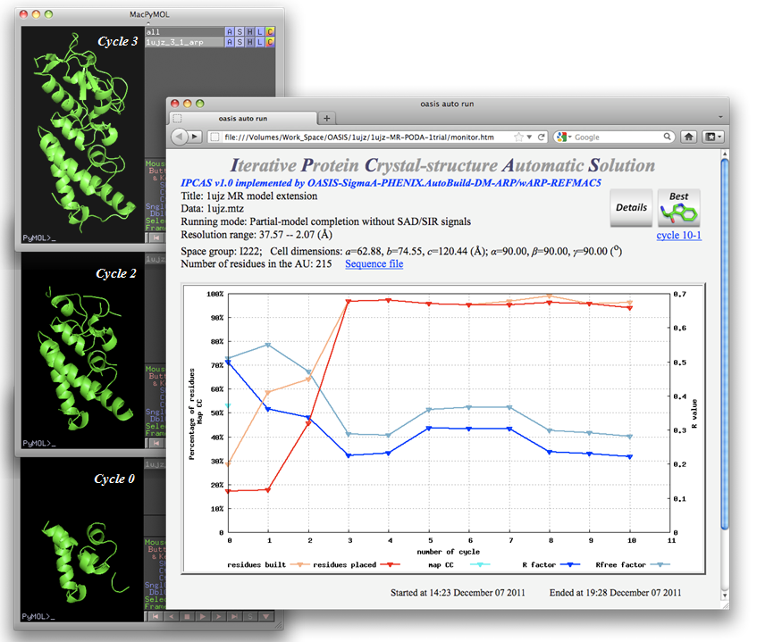
This example simulates a difficult MR (Molecular Replacement) case. The protein consists of two domains A and B in the asymmetric unit. The starting MR model corresponds to a part of A and amounts to ~20% of the whole structure. Data and parameters used in the calculation are shown on the control panel below.
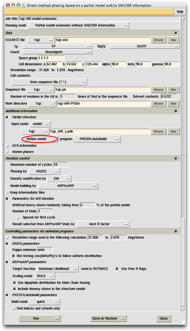
Right click the button marked with a red oval, you can get the following message:
The iteration results are shown below. Part of the growing process of the built model is given on the left of the figure. As is seen, a nearly complete structure model came already from cycle 3.
Back to TOP
Back to OASIS.html
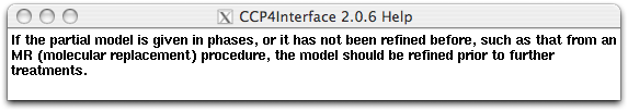
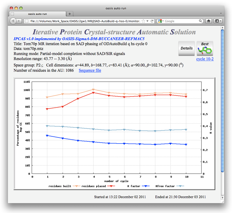
While the MR iteration is originally designed for MR-model completion, it is also efficient in the extension of partial structure models from a wide variety of sources. Examples from the present one onward are given to such kind of applications. In this example we take the Tom70p SAD model from cycle 0 of Example 2 as the starting model. This model contains ony helices and strands. Please note that while the starting model comes from SAD phasing, there were nothing with SAD signals in the following calculations. Data and parameters used in this example are shown below.

The resulting monitoring board is shown in the following. While the top-right button on it tells that the best model is from cycle 10-2, details on R factors and numbers of built residues and sequenced residues show that the best model should be that from cycle 8-4, which is nearly the complete structure as is shown by ribbon-model plots below the monitoring board.

Comparing the best model ("c" in the above ribbon-model plots) with that resulting from Example 2, it is seen that at least for the present example the combination of SAD and MR iteration is much better than the SAD iteration alone.
Unlike that in Example 4, in the present MR iteration there are 5 random trials in each cycle. Only results from the trial that leads to the smallest R factor (this is set on the control panel) will be passed onto the next cycle (see the following figure).
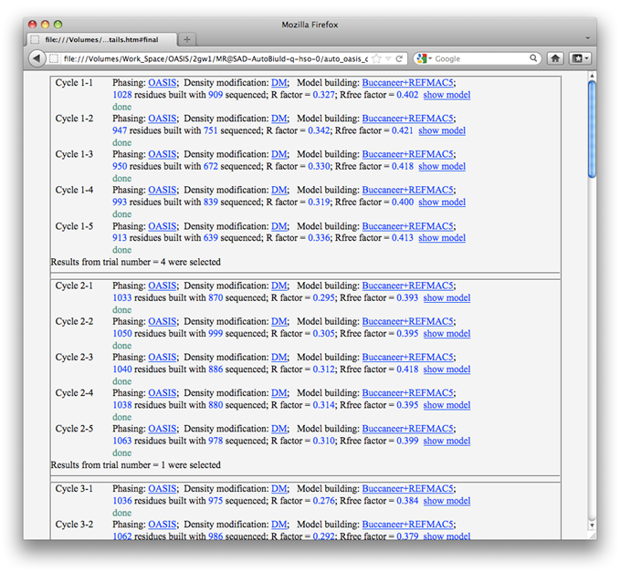
Upon finished running of each cycle, a message board like that in the following figure will pop-up listing details of the 5 trials, with one of them marked (selected) to be passed onto the next cycle. You have 5 minutes to change the selection manually. In order to force IPCAS continue running immediately, please click on the "confirm" button and reply "Allow" to the Internet Security warning.

Back to TOP
Back to OASIS.html
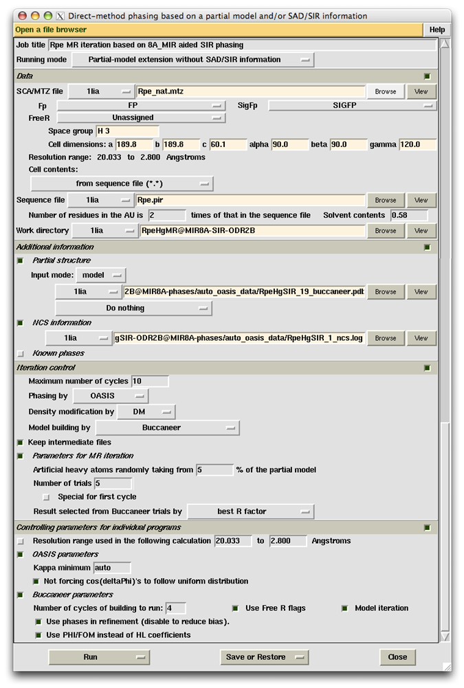
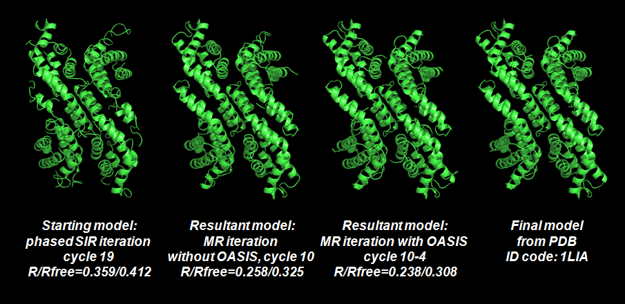
This example shows that the MR iteration is capable of improving a resultant model from SIR iteration. The starting model of this example comes from cycle 19 of the 8Å MIR-phased SIR iteration in Example 3. Control panel and monitoring board for the calculations are shown below.
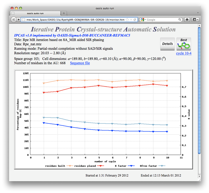
Both red and blue curves on the monitoring board indicate that the job was done successfully. Great improvement to the SIR-iteration result can be seen when comparing this monitoring board with that in Example 3.
Since the starting model is from cycle 19 of the 8Å MIR-phased SIR iteration, the question is: what would happen if the SIR iteration went on 10 more cycles? The answer is given in the following monitoring board, in which results of the extra 10 cycles of SIR iteration were recorded (see the portion with light blue background on the graph). From cycles 21 to cycle 30, the highest percentage of sequenced residues (shown with the red curve) is around 75%, while that for cycles 3 to 10 of the MR iteration (see the above figure) are nearly 100%. On the other hand, the lowest R factor (shown with the blue curve) in the following figure is above 0.35, while that in the MR iteration is below 0.25. This confirms that at least for the present example the combination of SIR and MR iterations is obviously better than SIR iteration alone.

MR iteration without OASIS:
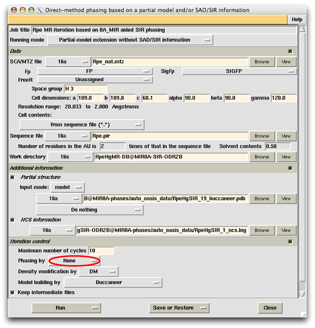
Provided the starting model is big enough, the MR iteration can also be done without OASIS. This is simlilar to the iteration of Fourier/least-squares refinement in small-molecule crystallography. To perform such calculations the only change to be made on the control panel is to replace OASIS by "None" when selecting the phasing program on the subframe "Iteration control", see the button marked with a red oval in the following figure. Right click the button will bring up a message board as shown below the figure of control panel.

Results according to the above control panel are recorded on the following monitoring board.
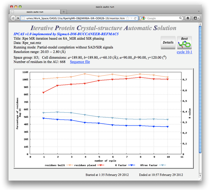
As is seen that the MR iteration without OASIS is quite successful. However the resultant model otained in this way is not as good as that from the MR iteration making use of OASIS. A detailed comparison together with the starting and final models are given below.
Back to TOP
Back to OASIS.html
Direct-method phase extension from a set of known phases at low resolution is another new feature of OASIS4.2. The P+ formular is used instead of the tangent formula for phase extension. Apart from the advantage of reducing the phase problem to a sign problem, the P+ formular is benificial to the combination of phase extension in reciprocal space and fragment extension in real space. In a different context, this new feature is achieved through the extension of MR iteration to accept known phases.
The protein Set 7/9 was originally solved by the MAD method at 2.7Å. This example shows that the protein could have been solved using 2.7Å structure-factor amplitudes with MAD signals to only 4.5Å resolution. The two figures below are the control panel for this purpose and the monitoring board resulted.

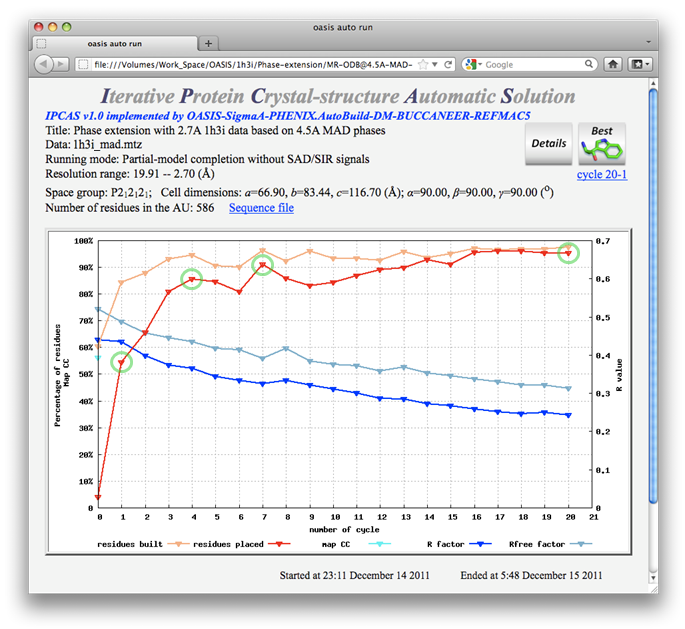
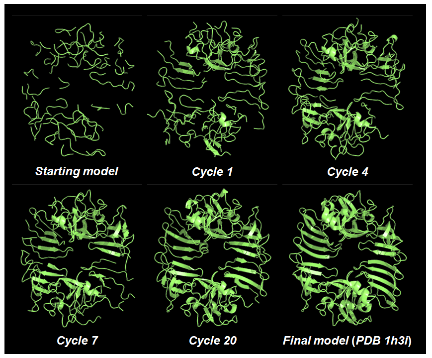
Ribbon models are plotted for cycles marked with green circles on the monitoring board together with the start and final models as is shown in the figure below. The sequenced residues in the best model (cycle 20) amount to ~95% of the whole structure.
Is OASIS a necessity? Withdrawing OASIS from the above process we got the following. As is seen the best model (shown on upper left of the following figure) becomes much more incomplete and fragmented. The maximum percentage of sequenced residues goes down from ~95% to ~70%, while the minimum R factor increased from ~0.25 to ~0.4. It is concluded that, at least for the present example, without OASIS the phase extension is far from successful.